Essentials of Chain Rule for Differentiation
This section describes some of the basics of chain rule for differentiation that we will use to describe automatic differentiation.
$$ \dfrac{ df(a \cdot b) }{dx} = b\dfrac{da}{dx} + a\dfrac{db}{dx} $$
For a function ‘f’ that is dependent on variables ‘ni(x)‘, the partial derivative w.r.t an independent variable ‘x’ can be written as shown below
$$ \dfrac{\partial f}{ \partial x} = \sum \dfrac{\partial f}{\partial n_{i} } \cdot \dfrac{ \partial n_i }{\partial x} $$
Types of Differentiation
Summarized here is a list of automated ways to compute the total or partial derivatives of a function computationally in an automated fashion.
- Symbolic differentiation
- Numerical Differentiation
- Finite differences
- Complex step derivatives
- Automatic Differentiation
- Forward-Mode Autodiff
- Reverse-Mode Autodiff
In this section we are going to skip both Symbolic Differentiation and Finite-Difference based Numerical differentiation since these are topics with which most are already familiar.
Numerical Differentiation with Complex-step Derivatives
In order to perform the differentiation we introduce the concept of an analytic function, i.e. functions that are infinitely differentiable and that can be smoothly extended into the complex domain. $$ f(x + ih) = f(x) + ihf^{\prime}(x) - \dfrac{h^{2}}{2}f^{\prime \prime} + O(h^3) $$ Taking the imaginary part on both sides we get $$ f^{\prime}(x) = \dfrac{imag(f(x + ih))}{h} + O(h^2) $$ NOTE: This can only be applied if the function is complex differentiable and satisfies the Cauchy-Riemann conditions as shown hereDual Numbers
Properties of Dual Numbers
Dual numbers are numbers of the type $$a + b\epsilon$$, where $$\epsilon$$ is a small number such that $$ \epsilon^2 = 0 $$ $$ \epsilon \longrightarrow 0 $$ A dual number is represented as a pair of floats. Additionally some important properties of dual numbers are $$ \lambda(a + b\epsilon) = \lambda a + \lambda b \epsilon $$ $$ (a + b\epsilon) + (c + d\epsilon) = (a + c) + (b + d) \epsilon $$ If 'h' is a function, the following important property holds $$ h(a + b \epsilon) = h(a) + bh^{\prime}(a) \epsilon $$ The above can be derived using the following polynomial P(x) $$ P(x) = p_{0} + p_1x + \mathellipsis + p_nx^n $$ $$ \Rightarrow P(a + b \epsilon) = p_0 + p_1(a + b \epsilon) + p_2(a + b \epsilon)^2 + \mathellipsis + p_n(a + b \epsilon)^n $$ $$ = p_0 + p_1a + p_2a^2 + \mathellipsis + p_na^n + p_1b \epsilon + 2p_2b \epsilon + \mathellipsis n p_na^{n-1} b\epsilon $$ $$ = P(a) + b \epsilon P^{\prime}(a) $$Using Dual Numbers to Compute the Derivatives
Let us consider a function f(x,y) = x2y + y + 2, we can compute the derivative $$f^{\prime}(x,y)$$ w.r.t ‘x’ by perturbing it as $$x + \epsilon$$ and taking the part accompanying epsilon as shown below
$$ f(x + \epsilon,y) = (x + \epsilon)^2y + y + 2 $$ $$ = x^2y + \epsilon^2y + 2\epsilon xy + y + 2 $$ $$ = x^2y + 2xy \epsilon + y + 2 $$ $$ \Longrightarrow \dfrac{\partial f(x,y)}{\partial x} = 2xy $$
Similarly $$\dfrac{\partial f(x,y)}{\partial y}$$ can be computed as
$$ f(x,y + \epsilon) = x^2(y + \epsilon) + (y + \epsilon) + 2 $$ $$ = x^2y + x^2\epsilon + y + \epsilon + 2 $$ $$ = x^2y + y + (x^2 + 1)\epsilon + 2 $$ $$ \Longrightarrow \dfrac{\partial f(x,y)}{\partial y} = x^2 + 1 $$
Computational Graphs
The properties of computational graphs can be summarized as follows:
- Any operation or a sequence of operations can be built as a directed acyclic graph with nodes and edges.
- Nodes represent either variables or constants and the direction of the edges represent dependencies.
- Any computation can be split into sub-operations such that each sub-operation can be represented using an operator and the list of operands it takes.
This will be used for building the Forward-Mode and Reverse-Mode Auto-differentiation algorithms as shown in the following sections.
Forward-Mode Autodiff
Figure 1 represents how to build a graph of computations for Forward-mode differentiation of f(3,4) w.r.t both ‘x’ by calculating $$f(x + \epsilon, 4)$$ In order to compute the partial derivative w.r.t ‘y’, the whole chain of computation needs to be recomputed by calculating $$f(3, 4 + \epsilon)$$
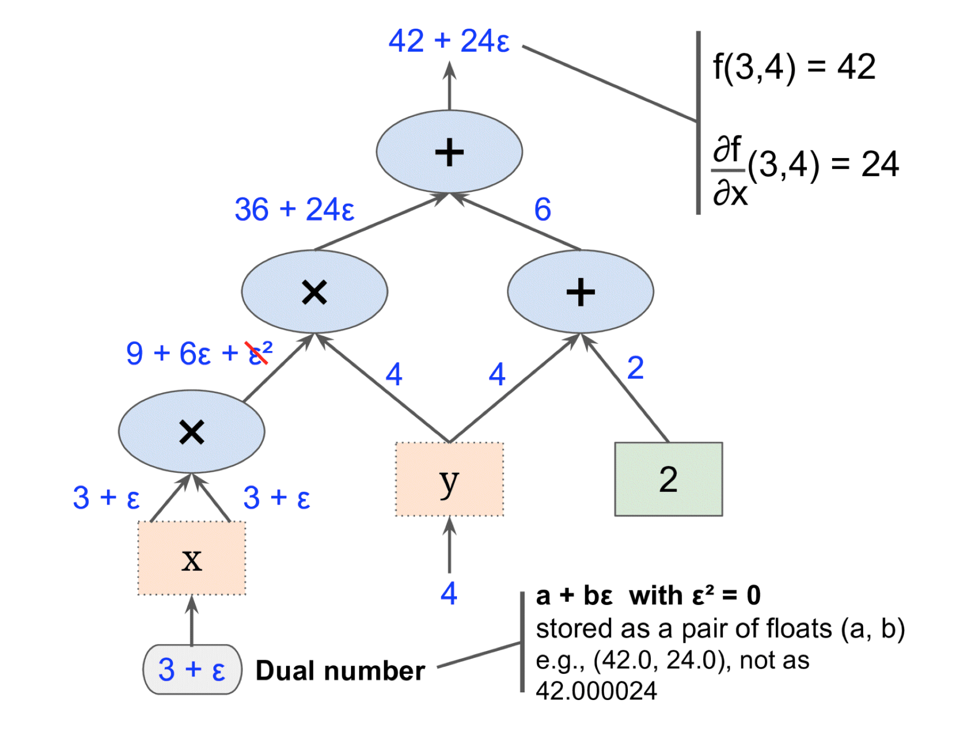
The problem with this approach is that for each independent variable, the function needs to be recalculated. Obviously this becomes expensive when there are a lot of independent variables, this is where Reverse-mode autodiff comes into play.
Reverse-Mode Autodiff
Reverse-mode autodiff can compute the derivatives w.r.t ‘n’ variables in two passes, irrespective of the number of variables. Reverse-mode autodiff is used in a lot of packages as a result of its efficiency. In the first pass, it computes the value of each node in the computational graph using a forward pass. In the second pass, the graph is traversed in the reverse direction from the top to the bottom. This is illustrated in Figure 2.
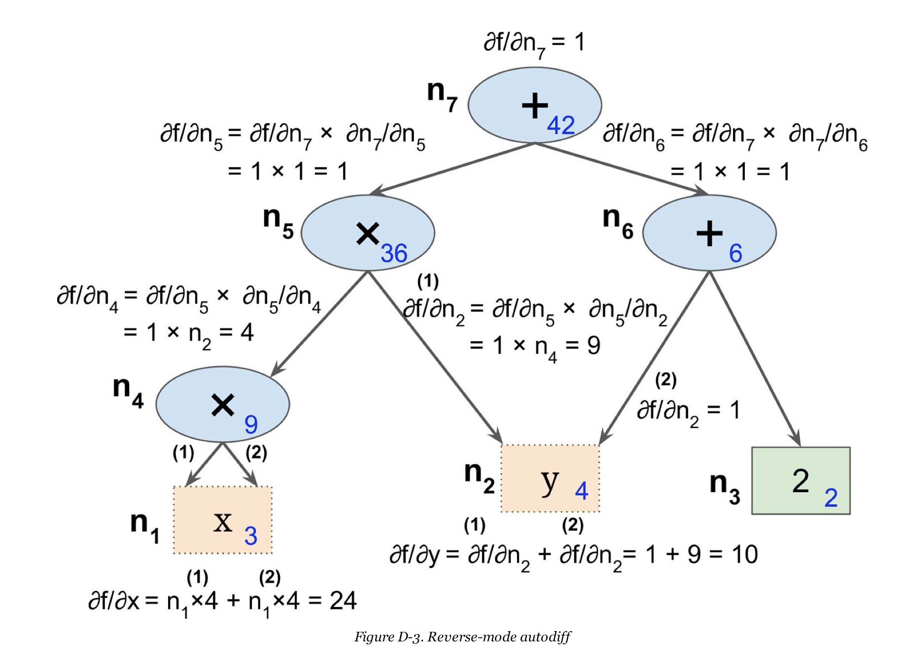
The process can be summarized as such:
- After the first pass as shown below, each node ni has a node value for a given set of input values to the function.
- As you traverse the graph from top to bottom, at node ni you build the partial derivative $$\dfrac{\partial f}{\partial n_i}$$ using the chain rule as shown in the first section. For e.g. looking at node 4 $$ \dfrac{\partial f}{\partial n_4} = \dfrac{\partial f}{\partial n_5} \cdot \dfrac{\partial n_5}{\partial n_4} $$
- For node 2( which is also y ), there are two nodes n5 and n6 that depend on it. Here, in accordance with the chain rule in the first section. $$ \dfrac{\partial f}{\partial n_2} = \dfrac{\partial f}{\partial n_5} \cdot \dfrac{\partial n_5}{\partial n_2} + \dfrac{\partial f}{\partial n_6} \cdot \dfrac{\partial n_6}{\partial n_2} $$
- Note here that each node ni only needs to know the partial derivative w.r.t the node directly beneath it along with the accumulated partial derivative $$\dfrac{\partial f}{\partial n_i}$$ to update the accumulated partial derivative.
- Once you fully traversed the graph, you will have the required partial derivatives for all variables.